This week, we are going to learn some advanced data structures for solving two very useful problems: The lowest common ancestor (LCA) problem and the range minimum query (RMQ) problem. You won't find these data structures in your standard library, so we will need to implement them ourselves.
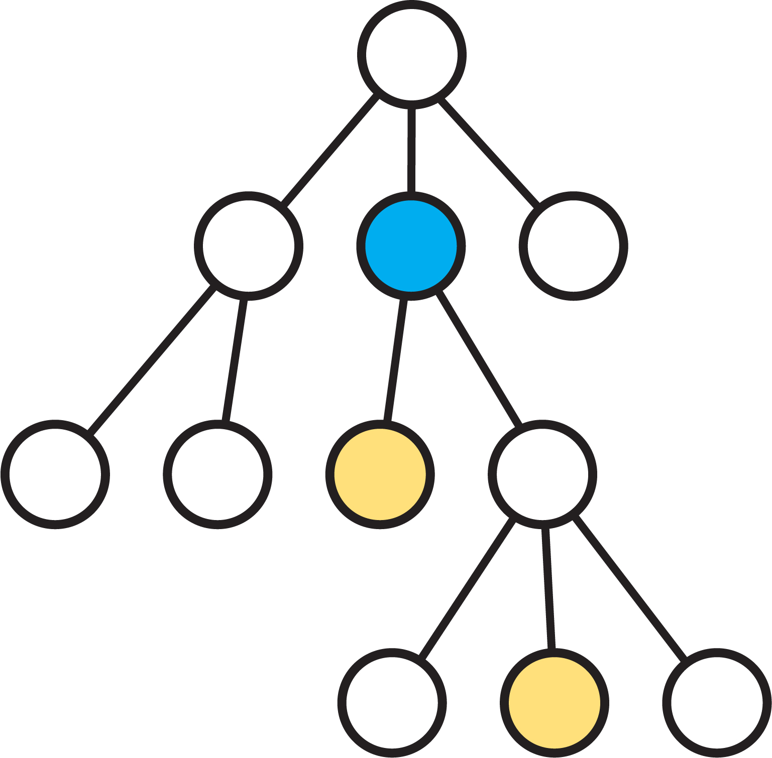
Given a rooted tree \( T \) and a pair of vertices \( u, v \), the lowest common ancestor of \( u \) and \( v \), which we will denote as LCA(\(u,v\)), is the lowest node in the tree that is both an ancestor of \( u \) and an ancestor of \( v \). See the following diagram for an example. The blue vertex is the LCA of the yellow vertices.
To get warmed up, let's start with a naive algorithm for computing LCAs. It seems pretty straightforward that we could simply walk up the tree from \( u \) and \( v \) until the two meet, then we are at the LCA. For instance, say we preprocess the tree and compute the level (distance from the root) of each vertex using a depth-first search, then we simply iterate by moving the lower vertex up one until the two meet.
// Precomputes levels
function precompute() {
  dfs(root, 0)
}

// Traverse the tree downwards from the vertex v
// Mark each vertex with its "level", i.e. its
// distance from the root
function dfs(v, lvl) {
  level[v] = lvl
  for (each child u of v) {
    dfs(u, lvl+1)
  }
}

// Compute the LCA of u and v
function lca(u, v) {
  while (u != v) {
    if (level[u] > level[v]) {
      u = parent[u]
    } else {
      v = parent[v]
    }
  }
  return u
}
This algorithm will compute the LCA of the vertices \( u, v \) after \( O(n) \) preprocessing to compute the levels. However, this algorithm will be really slow if the tree is very deep, because it may have to climb from the bottom of the tree all the way to the top. The complexity of a query is therefore \( O(h) \), where \( h \) is the height of the tree, which can be \( O(n) \) in the worst case. To be faster, we will need a smarter algoriithm.
The naive algorithm was slow because it could have to walk from the bottom to the top of a very tall tree. To overcome this, we will use the technique of binary lifting. The idea at its core is quite simple. At each vertex of the tree, instead of only knowing who the parent is, we also remember who the 2nd, 4th, 8th, ... ancestors are. We call these the binary ancestors of the vertex. This means that each vertex remembers \( O(\log(n)) \) of its ancestors, so we pay \( O(n \log(n)) \) space, but it will be worth it.
We can compute the binary ancestors in our preprocessing step with a depth-first search. The key observation that makes binary ancestors easy to compute is the following:
The kth binary ancestor of a vertex is the (k-1)th binary ancestor of its (k-1)th binary ancestor
We can use this fact to precompute all of the binary ancestors of all vertices in \( O(n \log(n)) \) time, as follows.
// Preprocess and compute binary ancestors
function preprocess() {
  for (each vertex v in the tree) {
    ancestor[v][0] = parent[v]
    for (k = 1 to log(n)) {
      ancestor[v][k] = -1
    }
  }
  dfs(root, 0)
  for (k = 1 to log(n)) {
    for (each vertex v in the tree) {
      if (ancestor[i][k-1] != -1) {
        ancestor[i][k] = ancestor[ancestor[i][k-1]][k-1]
    }
  }
}

// Traverse the tree downwards from the vertex v
// Mark each vertex with its "level", i.e. its
// distance from the root
function dfs(v, lvl) {
  level[v] = lvl
  for (each child u of v) {
    dfs(u, lvl+1)
  }
}
After this precomputation, we can use the binary ancestors to answer LCA queries in \( O(\log(n)) \) time with the following two-step idea. Start with the vertices \( u \) and \( v \).
First, we want to move the lower of the two vertices up the tree so that it is on the same level as the other one. We can do this in \( O(\log(n)) \) steps using the binary ancestors by noticing the following useful fact. Suppose without loss of generality that \( v \) is the lower of the two vertices. We want to move it \( \text{level}[v] - \text{level}[u] \) steps up. We can do this since every number can be written as a sum of powers of two (this is possible because we can write the number in binary). Therefore we can simply greedily move \( v \) up by the largest power of two that does not overshoot until we reach the desired level. This takes at most \( \log(n) \) time.
Now that \( u \) and \( v \) are on the same level, we use the following idea. We want to move both \( u \) and \( v \) up the tree as far as possible without them touching (which would be at their LCA). Suppose that their LCA is on level \( j \) and they are on level \( i \). Then we want to move them both up \( i - j \) levels. We can do this using the same trick as above, by greedily moving up by powers of two as long as they do not overshoot. The key observation that makes this work is that we can do this even without knowing the value of \( i - j \), because we can always check whether a move would be an overshoot by checking whether or not the corresponding ancestors are equal, and moving up only when they are not equal.
Here is some pseudocode to hopefully make this idea more concrete.
// Compute the LCA of u and v using binary lifting
function lca(u, v) {
  if (level[u] > level[v]) swap(u, v)
  for (k = log(n) - 1 to 0) {
    if (level[v] - pow(2, k) >= level[u]) {
      v = ancestor[v][k]
    }
  }
  if (u == v) {
    return u
  }
  for (k = log(n) - 1 to 0) {
    if (ancestor[v][k] != ancestor[u][k]) {
      u = ancestor[u][k]
      v = ancestor[v][k]
    }
  }
  return parent[u]
}
If \( n \) is not an exact power of two, be sure to round \( \log(n) \) up, not down, so that you compute enough ancestors. For an example implementation in C++, see this link. Their query algorithm is very slightly different to the one we describe, but uses the same underlying principles. Instead of performing our step 1 of moving the two vertices onto the same level, it simply moves the lower one up until it would become an ancestor of the first one, in which case it must have reached the LCA.
A common and useful application of LCA queries is for computing distances between vertices in trees. Suppose we have a weighted tree, i.e. the edges of the tree have weights, and we want to compute the lengths of paths between pairs of vertices. First, we solve an easier problem -- given a rooted, weighted tree, let's try to compute the lengths of paths from the root to any given vertex. This is much easier, we can simply perform a single depth-first search and aggregate the total weight of each path.
// Compute the weights of all root-to-vertex paths
function compute_path_weights() {
  dfs(root, 0)
}

function dfs(v, dist) {
  distance[v] = dist
  for (each child u of v) {
    dfs(u, dist + w(u,v))
  }
}
This will compute distance[\(v\)] for all vertices. We can now extend this to work for arbitrary paths in the tree. First, if our our tree is not already rooted, we can pick an aribtrary root, and perform the preprocessing step above to compute all root-to-vertex path lengths. Then, to compute the length of the path from \( u \) \( v \), we just notice that it is equal to $$ \delta(u, v) = \text{distance}[u] + \text{distance}[v] - 2 \times \text{distance}[LCA(u,v)]. $$ This is easy to see by drawing a tree and looking at the edges on the root-to-u path and the root-to-v path. Note that they contain all of the edges on the u-v path, but also all of the edges above their LCA twice. Hence the given formula should give us the correct value. Using this formula, we can therefore compute distances in trees in \( O(\log(n)) \) time per query (the cost of performing the LCA query) after having done \( O(n \log(n)) \) preprocessing for the binary ancestors.
For convenience, the depth-first search that computes the distances can be merged with the depth-first search that computes the levels for binary lifting, instead of writing two separate ones.
The range minimum query (RMQ) problem is the following: Given an array \( A \) and a pair of indices \( i, j \), we want to know the value of the smallest element of \( A \) between the indices \( i \) and \( j \). There are lots of data structures for dealing with RMQ. We will see two. One is super cool because it uses LCA and demonstrates a nice reduction between the two problems.
Here is how we can relate the two problems. Suppose we are given an array \( A \). We will build a tree on the elements of \( A \) like so: Take the minimum element, say \( A[i] \) of \( A \) and make it the root of the tree. Now take the subarrays \( A[0..i-1] \) and \( A[i+1...n-1] \) and build the same trees recursively, making them the left and right children of the root. This is called a cartesian tree. See the following diagram to illustrate.
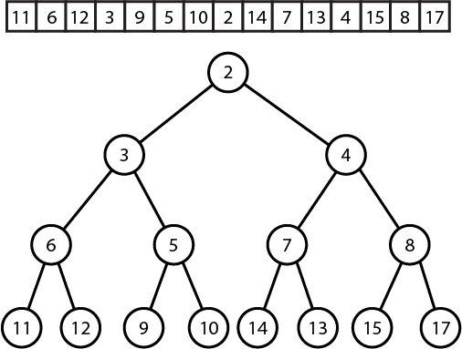
Observe that the RMQ of a range is just the LCA of the corresponding nodes! Therefore, if we can build a cartesian tree, we can use our LCA data structure to also solve the RMQ problem.
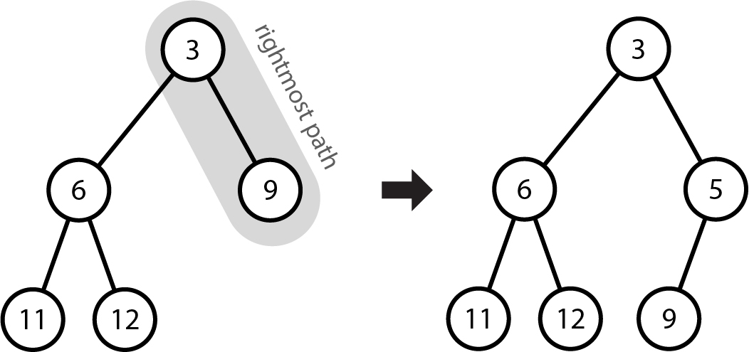
We can build a cartesian tree in linear time with the following idea. Let's scan the array left to right and maintain a cartesian tree of the elements that we have seen so far. The problem that we need to solve is: given a cartesian tree and one new element, how do we insert that new element into the tree? The key observation is this: Given a cartesian tree and a new element to insert, we will always insert that new element somewhere on the rightmost path of the tree. More specifically, notice that a cartesian tree satisfies the min-heap property, that is, every node has a value larger than its parent. So for each new node, we insert it into the rightmost path such that it stays in the correct order. The new element will be inserted as the right child of the existing node. If that node already had a right child, that subtree becomes the left child of the new node.
See the following diagram as an example. We have already built the tree for the elements 11, 6, 12, 3, 9, and now we wish to add 5. The rightmost path of the tree currently contains 3, 9, so we identify that 5 must go in between the two of those. 5 therefore becomes the right child of 3, and since 3 previously had 9 as a right child, that becomes the left child of 5.
To implement this, we can maintain a stack consisting of the current contents of the rightmost path. To insert something new, we can pop off the stack until we find the element that is less than what we want to insert (or if everything is greater than what we find, the new element becomes the new root). Note that once we insert a new element, all of the contents on the rightmost path that were larger than it are never on the rightmost path again, so it is safe to pop them off the stack and never look at them again. This means that every element is only ever pushed and popped once, so the algorithm runs in \( O(n) \) time. Here is some pseudocode to demonstrate. Note that we use the indices of the elements, rather than the elements themselves to index the nodes of the tree. Otherwise we wouldn't be able to use the result for anything useful.
// Given an array A, build a cartesian tree
// This consists in filling three arrays: parent, left_child, and right_child,
// and returning the root element. These are all with respect to indices, not
// values. A child of -1 indicates no child
function cartesian_tree(A[0...n-1]) {
  s = stack()
  root = -1
  for (i = 0 to n - 1) {
    next_largest = -1
    // Find the rightmost element that is smaller than A[i]
    while (s is not empty and A[s.top()] >= A[i]) {
      next_largest = s.pop()
    }
    // A[i] is inserted into the rightmost path
    if (s is not empty) {
      parent[i] = s.top()
      right_child[s.top()] = i
    }
    // A[i] becomes the new root
    else {
      left_child[i] = root
      root = i
    }
    // The previous contents of the rightmost path becomes A[i]'s left child
    if (next_largest != -1) {
      parent[next_largest] = i
      left_child[i] = next_largest
    }
    s.push(i)
  }
  return root
}
We can feed the resulting tree into our LCA data structure, and then answer RMQs on the range \( [i,j] \) by finding their LCA and returning the corresponding value.
An example implementation can be found here.
A final fun fact is that we can also reduce the other way. That is, if we have a data structure for RMQ, we can use that to solve the LCA problem.
Instead of reducing it to the LCA problem, an alternate way to solve RMQ is to use a data structure sometimes known as a sparse table. Sparse tables allow us to solve RMQ using \( O(n \log(n)) \) preprocessing, which is the same as the previous solution, but with just \( O(1) \) query time! The trick is to precompute the answer for \( n \log(n) \) carefully chosen intervals. Specifically, we precompute the answer for every interval of the form $$ [i, i + 2^k), \qquad 0 \leq i \leq n-1, \quad 0 \leq j \leq {\log(n)} $$ In other words, we have \( \log(n) \) intervals starting at each position, of sizes 1, 2, 4, 8, ... and so on. You can see the similar trick of using powers of two as in binary lifting. Powers of two are really useful like that.
Computing all of these naively would clearly take at least \( \Theta(n^2) \) time, but thankfully there is some nice substructure in these intervals. To compute the value of some interval of length \( 2^k \), note that it is simply two of the intervals of size \( 2^{k-1} \) joined together, so every interval can be computed in constant time! Specifically, the interval \( [i, i + 2^k) \) can be broken into \( [i, i + 2^{k-1}) \) and \( [i + 2^{k-1}, (i + 2^{k-1}) + 2^{k-1}) \). Here is some pseudocode to demonstrate.
// Fill in the sparse table data structure
// The sparse table is a log(n) * n size 2D array, where entry [k][i]
// gives the value of the minimum element in the interval [i, i + 2^k)
function sparse_table(A[0...n-1]) {
  for (i = 0 to n - 1) {
    sptable[0][i] = A[i]
  }
  for (k = 1 to log(n)) {
    for (i = 0 to n - pow(2, k)) {
      sptable[k][i] = min(sptable[k-1][i], sptable[k-1][i + pow(2, k-1)]
    }
  }
}
If \( n \) is not an exact power of two, like last time, we round \( \log(n) \) up to be safe. To perform a query, we observe that every interval \( [i,j] \) can be formed by combining two (not necessarily disjoint) intervals from the sparse table. Since it is okay to double up elements when computing the min, this is fine, and we can simply take the min of those two intervals to get the answer. Specifically, if we let \( k = \lfloor{\log(j - i + 1)}\rfloor \), the interval \( [i,j] \) is covered by the intervals \( [i, i + 2^k) \) and \( [j - 2^k + 1, (j - 2^k + 1) + 2^k) \).
// Query for the minimum element in the interval [i, j] (inclusive)
function RMQ(i, j) {
  k = floor(log(j - i + 1))
  return min(sptable[k][i], sptable[k][j - pow(2, k) + 1])
}
Be sure to round \( k \) down, not up, if the interval size is not a power of two, or you will include extra elements by mistake. You can see an example implementation here.
Lastly, note that the sparse table can easily be modified to answer other kinds of queries, like max, gcd, lcm, etc. It can not directly be used for sums, though, since the intervals used by the query might overlap.